Data Processing II

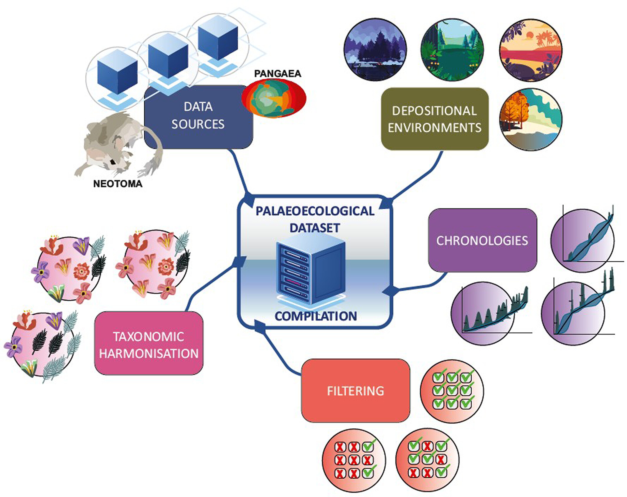
Data Processing II: Data Harmonization and Synthesis

Learning Objectives

In this session, we’ll walk through how to combine different deep time and modern datasets to answer questions that cross the palaeo-ecological divide. We’ll cover:

The power of harmonizing data from different sources
The considerations and complications that arise when combining datasets
How to source spatially explicit climatic data for the past and present, and how to look at relationships with fossil and modern occurrences
How to plan, write code for, and carry out projects covering multiple time frames

Plan for the Session

The session will be split into the following sections:

Introduction to harmonization and synthesis
Planning, setup, and finding your data
Building a workflow to merge datasets
Data visualisation and synthesis

Schedule

14:00–15:30

I. Introduction to Harmonization and Synthesis

So far, we’ve used R to carry out a variety of operations for acquiring and preparing palaeontological data. We can also use R to run analyses with the aim of answering specific research questions. We touched on this briefly during the last session when we looked at the latitudinal ranges of Crocodylia occurrences, but we can push our analyses further than that.

It will be of no surprise to anyone in this room that we are in the midst of a biodiversity crisis. Understanding and anticipating the changes that will occur to organisms, their communities, and the environments that they inhabit as a result of climate change and other anthropogenic stressors has emerged as a primary goal of our disciplines. Traditionally, modern ecologists have focused on studying current or recent historical processes to address questions related to biodiversity loss and the impacts of climate change, while palaeoecologists have studied long-term processes in the fossil record (Nieto-Lugilde et al. 2021). However, it is becoming increasingly clear that the answers to some of the most important questions relate to the fuzzy area between our modern and palaeo records:

Can past ecosystems be used as analogues for present-day ecosystems? Can we understand future changes to biodiversity by examining past losses?
What are the main drivers and consequences of collapse within communities and ecosystems?
When examining modern ecosystems, have crucial elements been lost? How can we set accurate baselines for conservation efforts?

Combining datasets spanning different timescales can help us address these questions. As you’ve seen earlier today, there are a wealth of available datasets that contain information about organisms and climate today and in the past, be that across shallow or deep time. Individually these datasets track processes that operate on different spatial and temporal scales. For instance, the figure below from Darroch et al. 2022 shows the potential drivers of geographic range in organisms across modern, historical and palaeontological timescales:

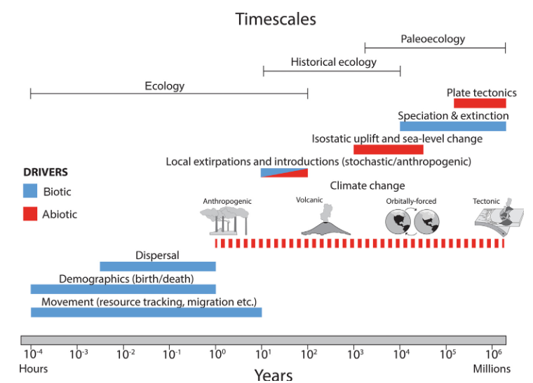
This figure emphasizes that ecological patterns such as geographic range are driven by processes operating on a continuum. The past and present are interconnected, and both can provide valuable information that can be combined to improve our understanding of underlying ecological processes. By developing approaches to harmonize data across timescales, we can begin to utilize this information to better understand drivers of ecological change, improve predictions of future biodiversity responses, and cross the palaeontological-ecological gap.

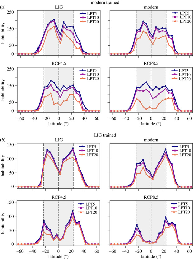
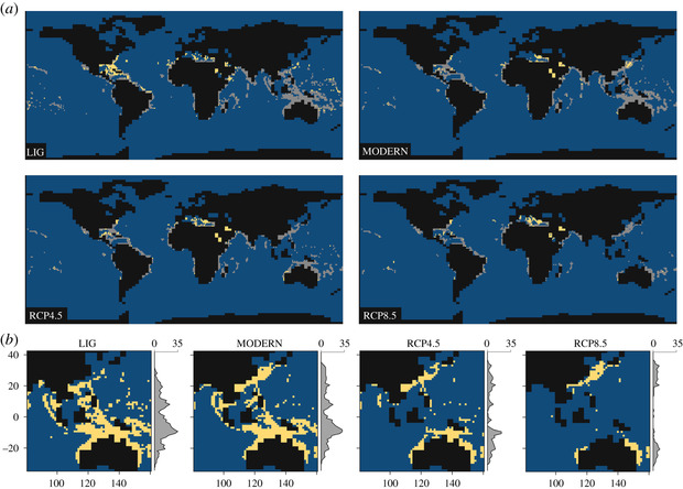
One research area that has particularly benefitted from the harmonization of palaeo and modern occurrence data is that of Species Distribution Models, or SDMs. These models correlate occurrences of species with climatic and environmental variables, and then use these associations to predict the distribution of that species across time and space. Consequently, they are frequently used to forecast species range shifts and understand potential losses in biodiversity as a result of future climate change. However, only including modern occurrences in these models excludes a vast amount of data of where organisms may have occupied in the past, running the risk of only predicting the occupied niche as opposed to gaining an understanding of the fundamental niche of a species (e.g., Veloz et al. 2012). This can have serious knock-on effects when attempting to predict the distribution of species under different climate scenarios. Consequently, studies have started to use the historical and palaeontological distribution of occurrences within these models. As you can see below, including coral occurrences from the last interglacial drastically changes the predicted habitability of corals under different IPCC forecasted climate scenarios (Jones et al. 2019):

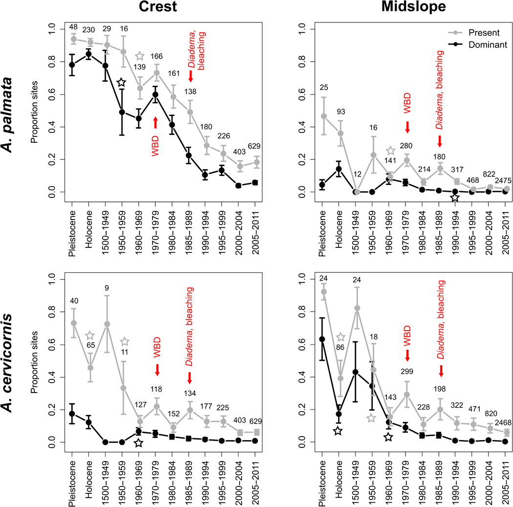
Another clear example of the harmonization of palaeo and modern data is in understanding long-term baselines of species abundances and distributions for conservation. This often involves combining records of presence or abundance that were collected in different ways over different timescales, and finding common currencies or other statistical approaches to align them. For example, by combining modern, historical, and palaeontological records of coral presence, (Cramer et al. 2020) examined the timing of coral decline in the Caribbean response to various regional and local stressors. They were able to track trends in coral abundance and community composition before recent ecological surveys, providing important baseline data for understanding the drivers of ongoing coral loss and where to target conservation and restoration efforts:

A final example synthesizes pollen data from cores to quantify rates of vegetation change over thousands of years in different regions, which sets the stage for investigating feedbacks between various anthropogenic and environvental drivers (Mottl et al. 2021). Databases like Neotoma contain a wealth of palaeoecological records such as this, alongside chronological information, that can be leveraged to reconstruct community change with relatively high temporal resolution in shallow time.

However, there are many considerations that have to be taken into account when carrying out this type of research, and a number of practical challenges that have to be overcome to ensure that the results we get are meaningful. Differences in spatial and temporal scales, data types, and various biases that impact our data sources all make this research difficult to carry out. Today, we are going to provide a brief introduction to this broad area of research, focusing in particular on the decisions that have to be made regarding our data and research approaches. Let’s dig in!

II. Planning, Setup, and Finding Your Data

Our Research Question

Our first step will be to define our research question, which will be framed around the dataset of Cenozoic Crocodylia that we worked on this morning. As mentioned previously, Crocs are an excellent group to use for studies comparing modern and deep time records: they have a very tight association with temperature, are well represented in the fossil record spatially and temporally, and many extant species are threatened by anthropogenic impacts including habitat loss and climate change.

In this section, we’ll aim to answer the following research question: How does the temperature range inhabited by Crocodylia in deep time compare to that seen in the present?

We’ll focus our deep time analysis on the Miocene, a climatically dynamic epoch in Earth’s history that can serve as an analog for future climate scenarios (e.g., Steinthorsdottir et al. 2020).

Making a Plan

Before we start, it’s helpful to write out a step-by-step plan of what we want to accomplish to ensure that the approach we’re taking and the code that we write will appropriately answer the question(s) that we are interested in. Think of this as a kind of “logical flow.” In other words, what are all the steps needed to get from our research idea to our finalised analysis? This can be as extensive as you wish and can be done in any fashion—even writing out your code or general approach on pen and paper! We’ll be doing this a few times today, so let’s start by considering our research question and what materials we’ll need to address it.

BREAKOUT SESSION 1

Organize yourselves into groups of 4-6 and take 10 minutes to discuss the following questions:

1. What datasets will we need to answer this question?

2. What issues might we encounter when sourcing, gathering, and working with these various datasets? How might these be addressed?

Solution

As we aim to compare the distributions of Crocodylia in deep time and the present, there are a couple of key datasets that we will require:

A spatially explicit dataset of modern Crocodylia
A spatially explicit dataset of Crocodylia in the deep time intervals we will assess
A spatially explicit dataset of modern climatic variables
A spatially explicit dataset of climatic variables for the deep time intervals we choose, likely generated from palaeo-climatic modelling

Heads Up!

Even at this first step, the decisions we make will have consequences for our research and findings. For example, our choice of datasets and how they are handled can impact our results. This will be a recurring theme throughout the session.

III. Building a Workflow to Merge Datasets

To help you get an idea of the process of using data from different sources, we’ll now walk through an example for how we might acquire and harmonize our climatic data. First, let’s make a plan of the steps we’ll take and some of the decisions we’ll need to consider along the way.

Decide which climate data to use. What will be most appropriate variables for the taxonomic group we are studying? Some potential choices might be:

The mean annual temperature
The mean annual range of temperature
The annual standard deviation of temperature
The temperature of the hottest or coldest quarter

Find a suitable source of data. We will need to find spatially explicit climatic data for each time interval we are interested in and acquire it in an appropriate format (.nc). What factors might we consider?

Availability of specifications listed above
Spatial resolution
Temporal resolution

Sort file structure. Ensure that your R project is set up appropriately and that the downloaded files are in an appropriate place to be used in your project, remembering to follow some of the guidance that we’ve covered earlier on today (e.g., ensuring there are raw versions of your data saved).
Load data. Read our data into R in an appropriate format to work with (e.g., raster). How might we do this? What packages might we need?
Check formatting and prepare for analysis. Ensure that the data are formatted appropriately. How might this impact our results or interpretations? What issues should we be aware of?

Do the data have the right extent for our research question and R pipeline, and can this be changed?
Are they at an appropriate spatial/temporal resolution, and can this be changed?
Are they in the right Coordinate Reference System?
Are they capturing the same climatic information?

In terms of our R code, we might want to break down our steps further:

Check the format of the data using the ‘class()’ function
Make a reference raster with appropriate resolution and extent
Ensure climate raster doesn’t have wrapping/extent issues, and rotate if necessary
Re-sample raster to our reference raster

Now that we have a basic plan, we can start to put it into action. Before we begin, we’ll need to install and load some packages that will allow us to work with our data:

# Install necessary packages
#install.packages("rgbif")
#install.packages("dplyr")
#install.packages("ggplot2")
#install.packages("palaeoverse")
#install.packages("raster")
#install.packages("sf")
#install.packages("geodata")
#install.packages("rnaturalearth")
#install.packages("ncdf4")
#install.packages("rgplates")

# Load packages
library(rgbif)
library(dplyr)


Attaching package: 'dplyr'

The following objects are masked from 'package:stats':

    filter, lag

The following objects are masked from 'package:base':

    intersect, setdiff, setequal, union

library(ggplot2)
library(palaeoverse)
library(raster)

Loading required package: sp


Attaching package: 'raster'

The following object is masked from 'package:dplyr':

    select

library(sf)

Linking to GEOS 3.12.1, GDAL 3.8.4, PROJ 9.4.0; sf_use_s2() is TRUE

library(geodata)

Loading required package: terra

terra 1.8.60

library(rnaturalearth)
library(ncdf4)
library(rgplates)

Now that’s done, let’s get cracking!

1. Deciding on climate data to use

As we want to link croc occurrences to temperature, we’ll need to find some spatially explicit climatic datasets for both the modern and deep time. This will mean that we can extract the temperature associated with the geographic location of those occurrences which can then be compared between our time intervals of interest.

We’ve also decided to keep things simple today and use the mean annual temperature to answer our research question, as this data is readily available in both palaeo and modern intervals. However, if we had more time, we might want to figure out how to find or calculate the temperature of the coldest quarter, as crocs are constrained physiologically by cooler temperatures. But that’s a challenge for another day. Now let’s find some data!

2. Finding a suitable source of data

2A. Palaeo data

After exploring several potential palaeo-climatic datasets, we’ve decided to use a dataset of global mean surface temperatures for the Phanerozoic (Scotese 2021), based on HadCM3L simulations and aligned with geochemical proxies like ∂18O. The data are available for 5-million-year intervals that cover our time period of interest (Miocene) and have a 1x1 degree (lat/long) resolution. The dataset is also publicly accessible via Zenodo: https://zenodo.org/records/5718392.

This climatic dataset offers decently high temporal resolution (for deep time), but one thing we’ll need to keep in mind is that the 5-million-year intervals don’t align perfectly with geological stages. This will come into play later when we start working with the occurrence data.

For our study, we’ll work with two files from this dataset: one covering 25-20 Ma and another covering 20-15 Ma. These data span warming intervals like the Mid Miocene Climatic Optimum and cooling intervals like the Oligocene-Miocene Climate Transition.

2B. Modern data

We’ll obtain our modern climatic data from WorldClim: https://www.worldclim.org/. WorldClim is a freely available set of global climate layers with a spatial resolution of about 1 square kilometer, which covers a variety of different climatic options. We can load these data directly into R using the geodata package, so no need to download anything for now!

Remember, to keep our climatic variables consistent we’ll also be working with mean annual temperature data, but we might have to do some fiddling to set that up (this will make more sense when we see the data!).

3. Sort file structure

Here we’d ensure that our downloaded palaeoclimate data are in an appropriate folder for our project. We’ll also set some default values to ensure that our spatial datasets conform with one another.

# Set spatial resolution
res <- 1

# Set spatial extent
e <- extent(-180, 180, -90, 90)

# Make generic raster using these values
ref_raster <- raster(res = res, ext = e)

4. Load data

4A. Loading palaeo-climatic data

We now need to load in our data, which is currently stored as a .nc file. This can be read into R as a raster using the raster package:

# Load in rasters of palaeoclimate for each time interval
raster2prep_15 <- raster(x = "015_tas_scotese02a_v21321.nc")
raster2prep_20 <- raster(x = "020_tas_scotese02a_v21321.nc")

4B. Loading modern climatic data

We can now use the geodata package to grab our modern climatic data. Whilst below we show you code to access this data directly within R, it can take a while to download. We’ve therefore also included it alongside the other materials for the workshop, which can be accessed HERE.

# Load data from WorldClim and make into raster
raster2prep_modern <- worldclim_global(var = "tavg", res = 10, path = tempdir())
raster2prep_modern <- as(raster2prep_modern, "Raster")

5. Check formatting and prepare for analysis

5A. Formatting palaeo-climatic data

First, lets have a look at our palaeo climate data and compare it to our reference raster:

# Examine our raster layers
raster2prep_15

class      : RasterLayer 
dimensions : 180, 361, 64980  (nrow, ncol, ncell)
resolution : 1, 1.005556  (x, y)
extent     : -180.5, 180.5, -90.5, 90.5  (xmin, xmax, ymin, ymax)
crs        : NA 
source     : 015_tas_scotese02a_v21321.nc 
names      : X015_tas_scotese02a_v21321 
zvar       : 015_tas_scotese02a_v21321

raster2prep_20

class      : RasterLayer 
dimensions : 180, 361, 64980  (nrow, ncol, ncell)
resolution : 1, 1.005556  (x, y)
extent     : -180.5, 180.5, -90.5, 90.5  (xmin, xmax, ymin, ymax)
crs        : NA 
source     : 020_tas_scotese02a_v21321.nc 
names      : X020_tas_scotese02a_v21321 
zvar       : 020_tas_scotese02a_v21321

ref_raster

class      : RasterLayer 
dimensions : 180, 360, 64800  (nrow, ncol, ncell)
resolution : 1, 1  (x, y)
extent     : -180, 180, -90, 90  (xmin, xmax, ymin, ymax)
crs        : +proj=longlat +datum=WGS84 +no_defs

As you can see, the resolution and extent of these rasters doesn’t quite match the reference one that we made above. We’ll have to resample our data to match our reference raster:

# Resample data to match our set extent and resolution
raster_resampled_15 <- resample(x = raster2prep_15, y = ref_raster)
raster_resampled_20 <- resample(x = raster2prep_20, y = ref_raster)

Finally, we can stack these rasters into one file, name them, and see what they look like:

# Stack rasters
scotese_temp <- stack(raster_resampled_15, raster_resampled_20)

# Name and plot rasters
names(scotese_temp) <- c("Burdigalian","Aquitanian")
plot(scotese_temp)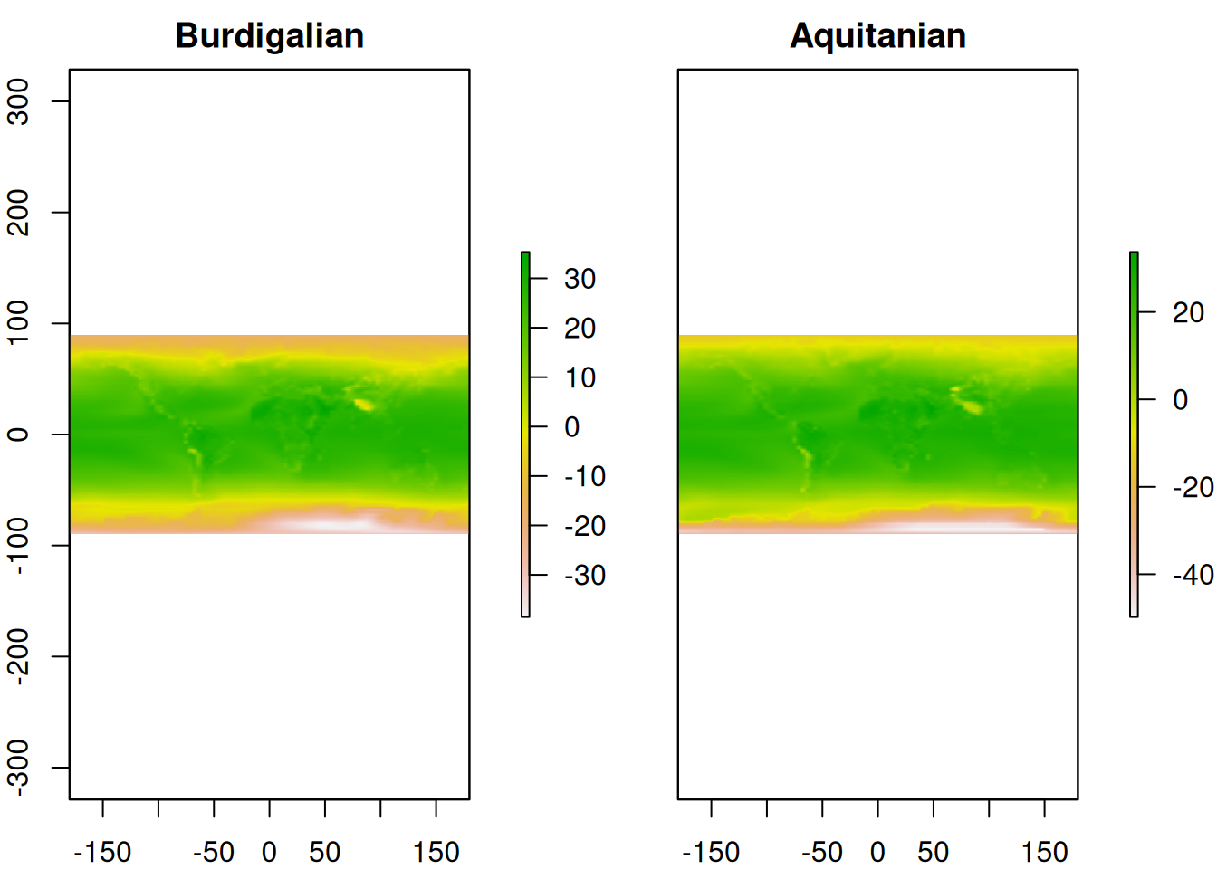

5B. Formatting modern data

Now let’s have a look at our modern data:

# Examine our modern raster:
raster2prep_modern

class      : RasterStack 
dimensions : 1080, 2160, 2332800, 12  (nrow, ncol, ncell, nlayers)
resolution : 0.1666667, 0.1666667  (x, y)
extent     : -180, 180, -90, 90  (xmin, xmax, ymin, ymax)
crs        : +proj=longlat +datum=WGS84 +no_defs 
names      : wc2.1_10m_tavg_01, wc2.1_10m_tavg_02, wc2.1_10m_tavg_03, wc2.1_10m_tavg_04, wc2.1_10m_tavg_05, wc2.1_10m_tavg_06, wc2.1_10m_tavg_07, wc2.1_10m_tavg_08, wc2.1_10m_tavg_09, wc2.1_10m_tavg_10, wc2.1_10m_tavg_11, wc2.1_10m_tavg_12 
min values :         -45.88400,         -44.80000,         -57.92575,         -64.19250,         -64.81150,         -64.35825,         -68.46075,         -66.52250,         -64.56325,         -55.90000,         -43.43475,         -45.32700 
max values :          34.00950,          32.82425,          32.90950,          34.19375,          36.25325,          38.35550,          39.54950,          38.43275,          35.79000,          32.65125,          32.78800,          32.82525

ref_raster

class      : RasterLayer 
dimensions : 180, 360, 64800  (nrow, ncol, ncell)
resolution : 1, 1  (x, y)
extent     : -180, 180, -90, 90  (xmin, xmax, ymin, ymax)
crs        : +proj=longlat +datum=WGS84 +no_defs

As you can see, although the extent matches our reference raster, these modern climatic data are considerably higher resolution than what we have available for our deep time data. But there’s something else going on: there’s 12 layers within this raster! This is because there’s a climatic layer for each month of the year. Therefore, we’ll have to calculate the mean temperature before we can use this for comparison:

# Calculate mean annual temperature
modern_mean <- calc(x = raster2prep_modern, fun = mean)

# Plot raster
plot(modern_mean)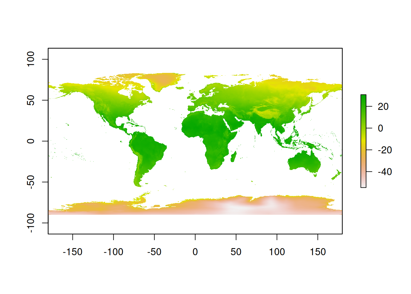

What issues might this higher resolution cause? What actions could we take to resolve this? What could we test?

BREAKOUT SESSION 2

Now it’s your turn to give it a go! Let’s spend the next 10-15 minutes to work through this same process for our occurrence data:

1. First, take a couple minutes to jot down a workflow for the fossil and modern occurrence data. Think about where you might find these data, if you’ll need to do any filtering, and how you might format them to enable fair comparisons across time with the climatic data that we just read into R. If you’re an experienced R user, you can also start to plan your code.

2. Then, get into the same groups you were in previously to discuss your approach. Where you might encounter potential pitfalls? What packages or approaches might make this process easier?

Solution

Let’s start by thinking about what we need from our occurrence datasets. To answer our question, we aim to compare Crocodylia occurrences in the past and present in relation to temperature data from the same geographic coordinates.

How do we get there? Let’s outline some potential steps:

Decide which occurrence data to use and where to source it. The PBDB Crocodylia dataset we’ve been working with contains occurrences that span our interval of interest. Where might we find a comparable dataset of modern occurrences? Earlier today, we learned about the Global Biodiversity Information Facility (GBIF). This could be a good source!
Filtering. We’ll need to do some filtering, for example to our time period of interest and to remove occurrences that have high uncertainty or aren’t comparable between the datasets. What other filtering criteria might we consider?
Cleaning. As we learned in the previous session, we’ll also want to spend some time cleaning and exploring our data.
Merging data. We’ll next want to combine our occurrence and climatic datasets to extract the mean temperature values at the same points in space and time as the occurrences. When doing this, what are some factors we need to consider? This might involving binning our data given differences in temporal and spatial resolutions and making some decisions about which taxonomic level to run our analysis. Along the way, we’ll likely need to think carefully about the dataframe structures and identify common data fields that are relevant for our study (time designations, taxonomy, coordinates, collection numbers, etc). We’ll also want to consider potential sampling biases that might influence our comparisons.
Data extraction and visualisation. At this point, we’ll have binned fossil and modern occurrences with geographic coordinates and associated temperature data. Returning to our question, this will allow us to determine whether the fossil occurrences cover a broader range of temperatures than the modern occurrences.

Let’s begin!

1. Sourcing occurrence data

1A. Organise fossil occurrence data

First, we’ll load in our palaeontological data. Luckily for us, we’ve already been working with a Crocodylia fossil occurrence dataset. We’ll use these data in our analysis. If you’ve not quite finished cleaning your dataset, you can find a cleaned version that’s ready for this next step HERE.

# Load cleaned fossil data for order Crocodylia that we worked on earlier
fossil_occ <- read.csv("cenozoic_crocs_clean.csv")

1B. Organise modern occurrence data

After looking at the number and coverage of available records, we’ve decided to use the GBIF data.

We’ll start by doing a quick data download using the rgbif package for the purposes of this exploratory exercise. Note that this method for retrieving occurrences has some limitations, and we’d want to do a formal download query before running our full analysis for publication. For that, you’d need to make a GBIF account.

Here’s how we can do this. Scroll down to load the dataset we’ve previously downloaded.

# Set taxa key to order Crocodylia
#crocodile_key <- name_backbone(name = "Crocodylia")$usageKey

# Download data
#modern_download <- occ_search(
  #taxonKey = crocodile_key,
  #hasCoordinate = TRUE, #needs to have coordinates
  #basisOfRecord = "PRESERVED_SPECIMEN", #keeping just preserved specimens for better comparability with the PBDB data
  #limit = 10000)  #adjust limit (if you set limit to 0, you can check the metadata to see how many records are available)

# Extract data
#modern_occ <- modern_download$data

# Extract metadata
#modern_meta <- modern_download$meta

For ease, here’s a csv of the raw data download:

# Load modern data
modern_occ <- read.csv("crocs_modern.csv")

Don’t forget!

Remember what we learnt in our session earlier: keep raw data raw! Make sure to always keep a copy of the raw data that you have used for your analyses, be that occurrence data or covariate data (such as climatic data).

2. Filtering

These datasets contain occurrences that are relevant to our research question, but they also contain occurrences that fall outside of the scope of our planned analysis. Let’s filter the datasets to just keep the relevant occurrences. What were some of the filtering criteria you brainstormed during the breakout session?

Data type: Note that we’ve already queried GBIF for just the preserved specimens to optimize comparability with the PBDB dataset. For instance, GBIF also contains fossil specimens, living specimens, and human observations that either aren’t entirely comparable with a fossil occurrence or don’t represent our modern time interval.
Taxonomic: We’ll run our analysis at the order level (Crocodylia) given taxonomic differences between the fossil and modern datasets at finer taxonomic levels (e.g., extinct taxa). That said, let’s just retain occurrences that have been identified at least to genus (i.e., removing indet. taxa from the fossil dataset) given uncertainty in their taxonomy.
Spatial: Our research question is posed at a global scale, so we can keep everything. However, we will still want to check for potential geographic outliers or inconsistencies while cleaning the data.
Temporal: We’ll constrain our palaeontological dataset to the same time intervals as our climatic dataset (25-15 Ma). Earlier, we downloaded Crocodylia occurrences for the whole of the Cenozoic, so we’ll need to do some filtering. Our modern dataset includes occurrences from the 1800s to today, whereas the WorldClim dataset starts at 1970, so we can also filter the occurrence dataset to that time range for consistency.

## PBDB filtering
fossil_occ_filter <- fossil_occ %>%
  dplyr::filter(accepted_rank == "genus" | accepted_rank =="species") %>% #taxonomic filtering
  dplyr::filter(max_ma<=25 & min_ma>=15) #temporal filtering

## GBIF filtering
modern_occ_filter <- modern_occ %>%
  dplyr::filter(!is.na(genus)) %>% #taxonomic filtering
  dplyr::filter(year >= 1970) %>% #temporal filtering
  dplyr::filter(coordinateUncertaintyInMeters < 10000 | is.na(coordinateUncertaintyInMeters)) #we could also remove data with uncertain geographic coordinates

This filtering step could have removed a fair amount of data. How many occurrences remain in each filtered dataset?

nrow(fossil_occ_filter)

[1] 102

nrow(modern_occ_filter)

[1] 2504

After filtering, we notice that there are far more modern occurrences than fossil occurences to potentially work with. How might we deal with this unequal sampling?

3. Cleaning

We’ll then want to explore and clean our data to check for outliers, inconsistencies, duplicates, and other potential issues.

Our fossil occurrence dataset has already gone through this process.

Practise Time! (optional)

Let’s spend a couple of minutes cleaning and familiarising ourselves with the GBIF data, applying what we learned in the previous session. For example, you might look at the range of latitudes represented by occurrences or check the taxa for spelling errors. You could plot them on a map to see if you notice any geographic oddities. Or you could check for duplicates. Alternatively, you can check out the GBIF webpage to see what’s available.

4. Merging

Now we come to the fun part. How do we align these data, which were sampled in different ways with different temporal and spatial resolutions and coverage? Note that the header names differ, and that the datasets contain variables reported in different ways (units, formats) and with different resolutions.

BREAKOUT SESSION 3

Return to your discussion groups and take 5 minutes to discuss the following questions:

1. What factors that might introduce bias when we try to make comparisons across these datasets?

2. What are some sources of uncertainty regarding the taxonomic, temporal, and spatial attributes of the data?

3. How might we address these potential confounds prior to analysis and/or what should we keep in mind as we’re interpreting our results?

As you discuss, you may find it helpful to return to your notes from Breakout Session 1.

Tip

The resolution and coverage of the data is likely one aspect that came up in your group discussions, both here and in Breakout Session 1. As we move forward, we’ll need to make some practical and philosophical decisions about how we bin the data given their varying resolutions. We’ll also want to consider the sensitivity of our results to these various decisions.

Let’s now have a group discussion about these taxonomic, temporal, and spatial considerations when endeavoring to make our datasets comparable.

4A. Taxonomy

We’ll be using higher-level taxonomic groups for our analysis. Let’s take a look to see what’s here.

# Fossil occurrences
table(fossil_occ_filter$family)


      Alligatoridae        Crocodylidae          Gavialidae NO_FAMILY_SPECIFIED 
                 18                  26                  18                  40

# Modern occurrences
table(modern_occ_filter$family)


Alligatoridae  Crocodylidae    Gavialidae 
         1933           492            79

We see that the same families are represented in our datasets (with the fossil occurrence dataset lacking some family-level classifications). If you were to look at the genera, you’ll notice some differences. If we wanted to run an analysis at a finer taxonomic level, what would be some key considerations or steps that we would need to take?

4B. Temporal Bins

Earlier, we noticed that our climatic data were available at 5-million-year intervals, which don’t align perfectly with geological stages. For example, our 25-20 Ma interval crosses the Chattian and Aquitanian stages and the 20-15 Ma interval crosses the Burdigalian and Langhian stages. On the other hand, each fossil occurrence has an associated age and interval range. We want to create time bins that roughly correspond with our climate layer so we can look at occurrences in relation to the temperature reconstructions. How might we approach this?

First, let’s take a look at the temporal distribution of our fossil occurrences.

head(x = tax_range_time(occdf = fossil_occ_filter, 
               name = "occurrence_no",
               min_ma = "min_ma", 
               max_ma = "max_ma", 
               plot = TRUE))

     taxon taxon_id max_ma min_ma range_myr n_occ
10  643927        1   16.9  15.98      0.92     1
16  650903        2   16.9  15.98      0.92     1
29  742606        3   16.9  15.98      0.92     1
30  742607        4   16.9  15.98      0.92     1
31  742608        5   16.9  15.98      0.92     1
65 1193267        6   16.9  15.98      0.92     1

axis_geo(intervals = "stages")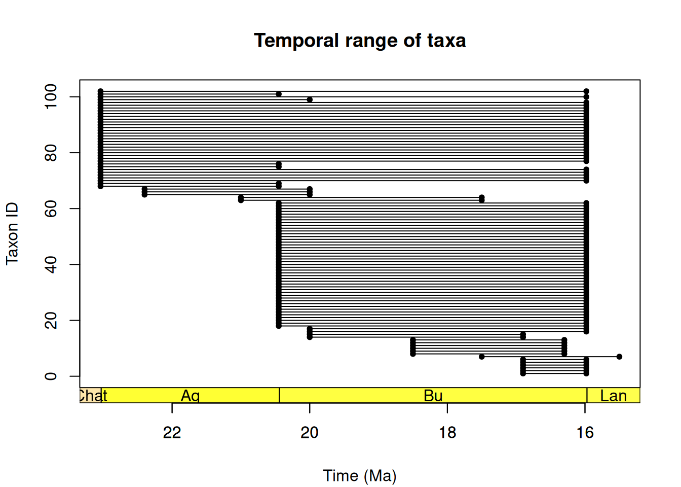

One option would be to bin the data by stage and use those as proxies for our 5-million-year climatic intervals. Another approach might be to make near-equal-length bins within the 25-15 Ma range, and then assign occurrences to those bins. Let’s try that latter approach here.

# Generate time bins of ~5 million years within 25 and 15 Ma
bins <- time_bins(interval = c(15,25), 
                  rank = "stage",
                  size = 5, #here's where we specify the equal-length bins to approximate the resolution of our climatic data
                  scale = "GTS2020",
                  plot = TRUE)

Target equal length time bins was set to 4.67 Myr. 
Generated time bins have a mean length of 4.67 Myr and a standard deviation of 2.02 Myr.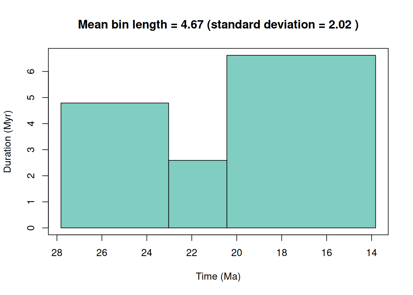

# Check bins
head(bins)

  bin max_ma mid_ma min_ma duration_myr grouping_rank             intervals
1   1  27.82 25.425  23.03         4.79         stage              Chattian
2   2  23.03 21.735  20.44         2.59         stage            Aquitanian
3   3  20.44 17.130  13.82         6.62         stage Langhian, Burdigalian
   colour  font
1 #80cdc1 black
2 #80cdc1 black
3 #80cdc1 black

There are also a couple methods that we could use to bin the occurrences. Let’s test out two methods here to see how they differ. Hopefully you’re starting to get a sense of how these various decisions might propagate to affect our results.

# `mid` method = uses the midpoint of age range to bin the occurrence
fossil_occ_mid <- bin_time(occdf = fossil_occ_filter,
                      bins = bins,
                      method = 'mid')

# `majority` method = bins an occurrence into the bin which it most overlaps with
fossil_occ_maj <- bin_time(occdf = fossil_occ_filter,
                      bins = bins,
                      method = 'majority') 

# Compare the bin assignments
bin_comparison <- fossil_occ_mid[c('occurrence_no','bin_assignment','n_bins')] %>% 
  left_join(fossil_occ_maj[c('occurrence_no','bin_assignment','n_bins')],by='occurrence_no') %>% 
  mutate(agreement = case_when(
    bin_assignment.x == bin_assignment.y ~ "yes"
  ))

In this case, they actually match up! Since these approaches yielded the same results, we’ll use the ‘maj’ dataset moving forward.

# Renaming
fossil_occ_bin <- fossil_occ_maj

# How many occurrences per bin?
table(fossil_occ_bin$bin_assignment)


 2  3 
 9 93

We see that most of the data falls into bin 3 (20.44-13.82 Ma, midpoint=17.130 Ma), with some occurrences in bin 2 (23.03-20.44 Ma, midpoint=21.735 Ma). We note that:

Bin 2 overlaps with our 25-20 Ma climate raster
Bin 3 overlaps with our 20-15 Ma climate raster

Our GBIF dataset already contains just modern data, which overlaps with our WorldClim climate layer, so no additional binning is needed.

OK, so now we have some temporal bins to facilitate our comparisons with the climatic data.

4C. Spatial Bins

We also observed that the spatial resolution of the climatic data differed between the past and present. Additionally, the uncertainties in the coordinates for our modern and fossil occurrences differ, especially since we’ll need to rely on plate models to palaeorotate the geographic positions of our fossil occurrences. How might we deal with this?

Like before, let’s take a look at the spatial distribution of our fossil occurrences.

# Load in a world map
world <- ne_countries(scale = "small", returnclass = "sf")

# Plot the geographic coordinates of each locality over the world map
ggplot(fossil_occ_bin) +
  geom_sf(data = world) +
  geom_point(aes(x = lng, y = lat)) +
  labs(x = "Longitude (º)",
       y = "Latitude (º)")+ 
  theme_void()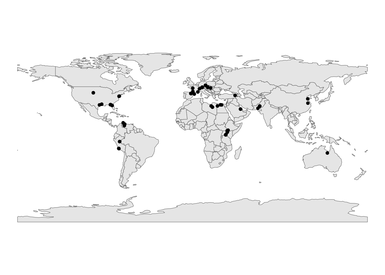

But wait, remember that we need to palaeorotate our coordinates before we proceed! We could run a couple different plate models to check the sensitivity, but for now we’ll just use the PALEOMAP rotation, which will also match up to our palaeo-climatic data.

# Palaeorotation
fossil_occ_bin_rot <- palaeorotate(fossil_occ_bin,
                                   lng = "lng",
                                   lat = "lat",
                                   age = "bin_midpoint", 
                                   model  = "PALEOMAP")

PALEOMAP

Heads Up!

Whilst the palaeorotate function is incredibly useful, the GPlates API can sometimes get overloaded with requests. If that happens, we can always use the palaeorotations included within the PBDB download. We’ll just have to rename the columns!

# Rename palaeorotation columns
rename(fossil_occ_bin_rot, p_lat = paleolat, p_lng = paleolng)

After some cleaning, we can then plot our rotated occurrences on a palaeogeographic map (here we’re going to use our bin 3):

# Remove NAs
fossil_occ_bin_rot <- fossil_occ_bin_rot %>%
  dplyr::filter(!is.na(p_lng) & !is.na(p_lat))

# Use the rgplates package to reconstruct a palaeogeographic map
coastlines <- reconstruct("coastlines", age=15, model="PALEOMAP")

# Plot palaeorotated coordinates for bin 3
fossil_occ_bin_rot %>%
  dplyr::filter(bin_assignment == 3) %>%
  ggplot() +
  geom_sf(data = coastlines) +
  geom_point(aes(x = p_lng, y = p_lat)) +
  labs(x = "palaeolongitude (º)",
       y = "palaeolatitude (º)")+ 
  theme_void()

For comparison, let’s also plot the modern occurrences.

# Load in a world map
world <- ne_countries(scale = "small", returnclass = "sf")

# Plot the geographic coordinates of each locality over the world map
ggplot(modern_occ_filter) +
  geom_sf(data = world) +
  geom_point(aes(x = decimalLongitude, y = decimalLatitude)) +
  labs(x = "Longitude (º)",
       y = "Latitude (º)")+ 
  theme_void()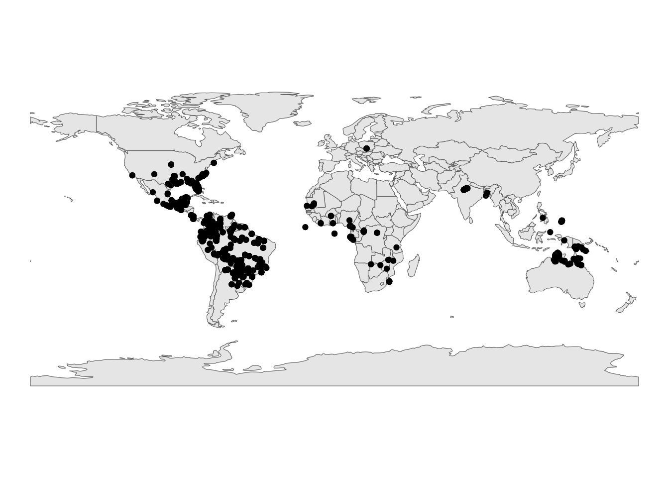

Looking at these spatial representations of the data, we can really visualise the difference in sampling effort. How might we account for the spatial structure of the data in our analysis?

Another challenge stems from aligning these occurrences with the spatially explicit climate layers. A simple approach would be to extract the mean temperature value at each coordinate. Alternatively, we might consider adding a bit of a buffer around each coordinate to incorporate geographic uncertainty and variation in the climatic data. A third, albeit more complex approach, would be to assign the occurrences to spatial bins so we can match them up to the climate layers (e.g., check out the bin_space function in the palaeoverse package). We’d also need to resolve the difference the spatial resolutions between the past and present climatic data, potentially by coarsening the modern dataset. We’ll keep things simple and show the first approach here.

Now moving onto the final section: using the combination of these datasets to carry out our analysis and visualise our results!

IV. Data Extraction and Visualisation

We’re nearly there folks. It’s time to put all these data sources together to answer our research question!🥁

We have our data binned to match the climate layers, so let’s create separate datasets for each time bin.

# 25-20 Ma climate interval
points_20 <- fossil_occ_bin_rot %>%
  dplyr::filter(bin_assignment == 2)

# 20-15 Ma climate interval
points_15 <- fossil_occ_bin_rot %>%
  dplyr::filter(bin_assignment == 3) 

# Modern interval (whole dataset)
points_mod <- modern_occ_filter

Next, let’s set up our points and ensure they’re on the same coordinate system. Recall that this was one of the things we wanted to check when we outlined our workflow for the climatic data at the beginning of the session.

# Turn points into spatial features
points_sf_20 <- st_as_sf(x = points_20, coords = c("p_lng", "p_lat"))
points_sf_15 <- st_as_sf(x = points_15, coords = c("p_lng", "p_lat"))
points_sf_mod <- st_as_sf(x = points_mod, coords = c("decimalLongitude", "decimalLatitude"))

# Set coordinate system (WGS84) for occurrences
st_crs(points_sf_20) <- st_crs(4326)
st_crs(points_sf_15) <- st_crs(4326)
st_crs(points_sf_mod) <- st_crs(4326)

We’re now ready to extract the climatic data at each coordinate!

# Past temperature (Scotese 2022)
scotese_temp_20 <- raster::extract(x = scotese_temp$Aquitanian, 
                           y = points_sf_20, 
                           sp = TRUE, 
                           cellnumbers = TRUE)

scotese_temp_15 <- raster::extract(x = scotese_temp$Burdigalian, 
                                     y = points_sf_15, 
                                     sp = TRUE, 
                                     cellnumbers = TRUE)

# Modern temperature (WorldClim)
modern_temp <- raster::extract(x = modern_mean, 
                                     y = points_sf_mod, 
                                     sp = TRUE, 
                                     cellnumbers = TRUE)

Let’s take a look. How does the temperature range inhabited by Crocodylia in deep time compare to that seen in the present?

# Aquitanian range (25-20 Ma)
range(scotese_temp_20$Aquitanian, na.rm=T)

[1] 18.43755 26.87847

diff(range(scotese_temp_20$Aquitanian, na.rm=T))

[1] 8.440919

# Burdigalian/Langhian range (20-15 Ma)
range(scotese_temp_15$Burdigalian, na.rm=T)

[1] 14.28417 33.11024

diff(range(scotese_temp_15$Burdigalian, na.rm=T))

[1] 18.82607

# Modern range
range(modern_temp@data$layer, na.rm=T)

[1]  8.368937 30.550188

diff(range(modern_temp@data$layer, na.rm=T))

[1] 22.18125

Finally, let’s plot the data.

# Organise data for plotting
palaeo_temp <- rbind(data.frame(Bin = rep("Burdigalian", length(scotese_temp_15$Burdigalian)), #
                           Temperature = scotese_temp_15$Burdigalian), 
                      data.frame(Bin = rep("Aquitanian", length(scotese_temp_20$Aquitanian)), 
                                  Temperature = scotese_temp_20$Aquitanian),
                      data.frame(Bin = rep("Modern", length(modern_temp@data$layer)), 
                                  Temperature = modern_temp@data$layer))

# Make box plot of temperature
ggplot(palaeo_temp, aes(x = Bin, y = Temperature)) +
  geom_jitter(color="gray80",size=2,alpha=0.5)+
  geom_boxplot(width=0.5,alpha=0.7,outlier.shape = NA)+
  labs(x="Time interval", y="Temperature (ºC)")+
  theme_bw()

Warning: Removed 3 rows containing non-finite outside the scale range
(`stat_boxplot()`).

Warning: Removed 3 rows containing missing values or values outside the scale range
(`geom_point()`).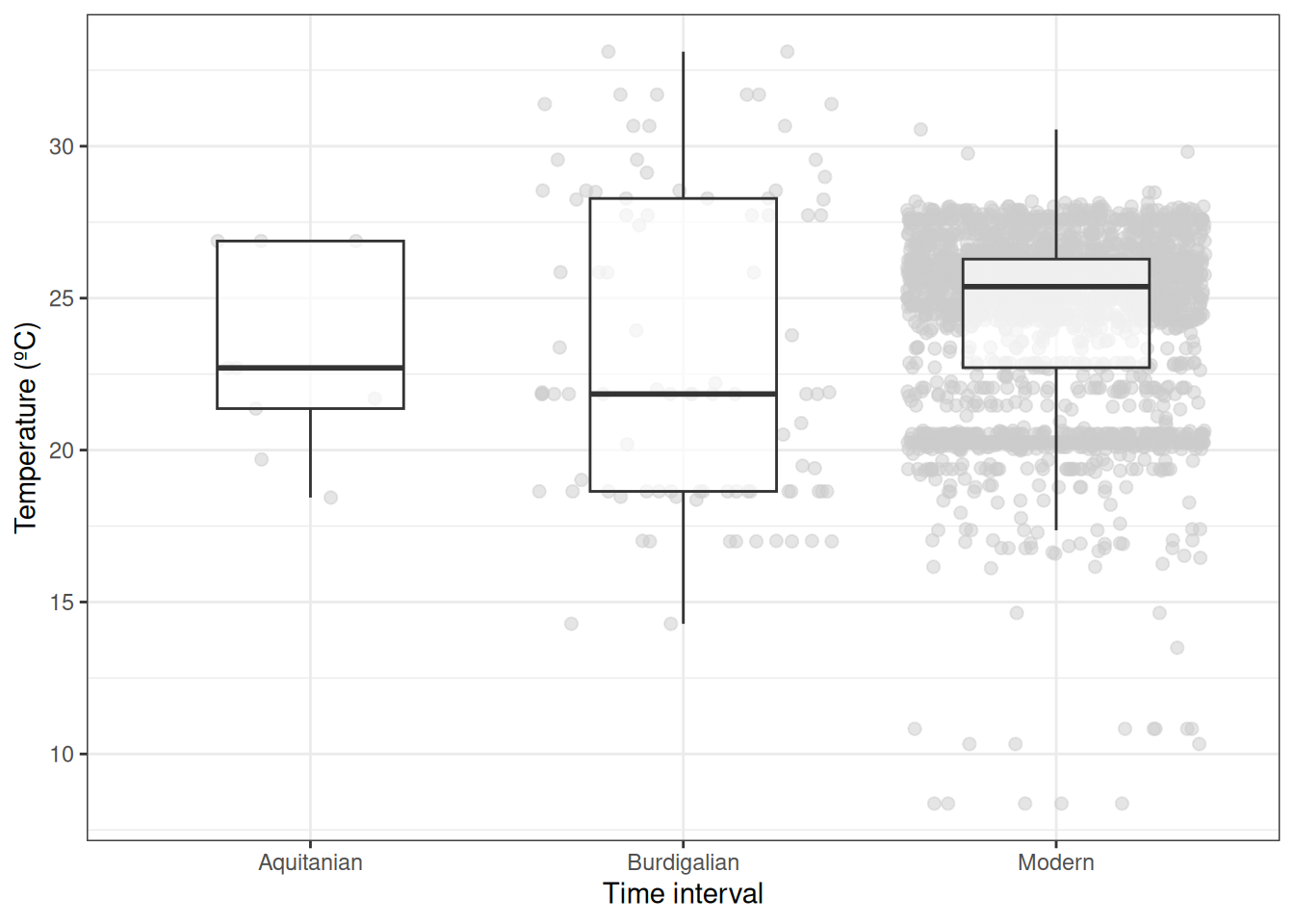

When looking at the better sampled intervals in particular, we find that the mean temperature range of Crocodylia occurrences was quite similar between the Miocene and Modern. How might we interpret our results? How might this interpretation be shaped by the caveats we pointed out along the way?

Ultimately, our goal was to provide a workflow for merging different types of datasets and thinking critically about some of the caveats that arise when doing so. These taxonomic, spatial, and temporal considerations are critical to address and report in palaeobiological and palaeoecological research in general—but particularly in studies aiming to cross the palaeontological-ecological gap. We hope you can adapt and learn from this script as you venture forward with your own exciting research questions and datasets!

References

Cramer, K.L., Jackson, J.B., Donovan, M.K., Greenstein, B.J., Korpanty, C.A., Cook, G.M., & Pandolfi, J.M. (2020). Widespread loss of Caribbean acroporid corals was underway before coral bleaching and disease outbreaks. Science Advances, 6(17), eaax9395.

Darroch, S.A., Saupe, E.E., Casey, M.M. and Jorge, M.L. 2022. Integrating geographic ranges across temporal scales. Trends in Ecology & Evolution, 37(10), 851-860.

Flantua, S.G., Mottl, O., Felde, V.A., Bhatta, K.P., Birks, H.H., Grytnes, J.A., … & Birks, H.J.B. (2023). A guide to the processing and standardization of global palaeoecological data for large‐scale syntheses using fossil pollen. Global Ecology and Biogeography, 32(8), 1377-1394.

Jones, L.A., Mannion, P.D., Farnsworth, A., Valdes, P.J., Kelland, S.J. and Allison, P.A. (2019). Coupling of palaeontological and neontological reef coral data improves forecasts of biodiversity responses under global climatic change. Royal Society Open Science, 6(4), 182111.

Mottl, O., Flantua, S.G., Bhatta, K.P., Felde, V.A., Giesecke, T., Goring, S., … & Williams, J. W. (2021). Global acceleration in rates of vegetation change over the past 18,000 years. science, 372(6544), 860-864.

Nieto-Lugilde, D., Blois, J.L., Bonet-García, F.J., Giesecke, T., Gil-Romera, G. and Seddon, A. (2021). Time to better integrate palaeoecological research infrastructures with neoecology to improve understanding of biodiversity long-term dynamics and to inform future conservation. Environmental Research Letters, 16(9), 095005.

Scotese, C.R., Song, H., Mills, B.J. and van der Meer, D.G. (2021). Phanerozoic palaeotemperatures: The earth’s changing climate during the last 540 million years. Earth-Science Reviews, 215, 103503.

Steinthorsdottir, M., Coxall, H.K., De Boer, A.M., Huber, M., Barbolini, N., Bradshaw, C.D., Burls, N.J., Feakins, S.J., Gasson, E., Henderiks, J. and Holbourn, A.E. (2021). The Miocene: The future of the past. palaeoceanography and palaeoclimatology, 36(4), e2020PA004037.

Valdes, P.J., Scotese, C.R. and Lunt, D.J. 2020. Deep ocean temperatures through time. Climate of the Past Discussions (2020). 1-37.

Veloz, S.D., Williams, J.W., Blois, J.L., He, F., Otto‐Bliesner, B. and Liu, Z. (2012). No‐analog climates and shifting realized niches during the late quaternary: implications for 21st‐century predictions by species distribution models. Global Change Biology, 18(5), 1698-1713.